3. SOFTWARE architecture
3.1 PRINCIPLE AND BLOCK DIAGRAMS

3.1.1 Reminder on the general principles of the ICI inversion system
3.1.2 General Principle of software subdivision
3.1.3 CMS choices

3.5.1 files for a PASS processing
3.5.2 files for the BASE_METEO creation
3.5.3 Files for the BASE_PROFIL initial library
3.5.4 MONITORING files
3.5.5 GRAPHIC files

1. SOFTWARE architecture
 
1. PRINCIPLE AND BLOCK DIAGRAMS

The general functional principles of the ICI application are described in detail in [Ref 4] and recalled in this section. Software subdivision is however organized in a slightly different way and the general subdivision principles are listed.
 

 
1. Reminder on the general principles of the ICI inversion system

The purpose of the ICI inversion system is to rebuild the vertical structure of the atmosphere in temperature and moisture. This is done using the radiative transfer equation inversion method, on the basis of the observations given by the sounders, each channel viewing a different region of the atmosphere.
Diagram 1 shows the main functions of the ICI inversion system.

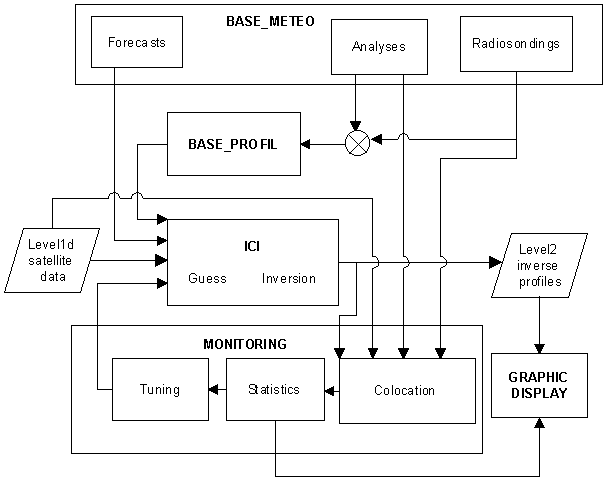
Diagram -1: Description of the ICI inversion processing system
The ICI system reads level1d TOVS/ATOVS incoming data that are navigated, temperature calibrated, mapped on the HIRS grid and documented after AAPP pre-processing. The maps that are presently being developed are the MSU on the HIRS grid for TOVS and the AMSU-A and AMSU-B on the HIRS grid for ATOVS. The main information associated with each HIRS fov are on the one hand the surface type (land/sea/mixed) and the altitude originating from topographic files and on the other hand the cloud cover and the skin surface temperature originating from the AVHRR cloud mask, and specifically for ATOVS, rainfall surface type flags originating from the AMSU preprocessing.
Preprocessing scientific processes are described in Ref [3] Vol.1. A detailed description of the AAPP output level1 file format is available in document [2] Vol.2.
ICI inversion software files are sequential access binary files with one record per situation containing the level1d incoming data, environment data, surface weather forecasts, the atmospheric profile used for initializing the inversion as well as the restituted profile. A detailed description of the format is given in chapter 3.5.
The inversion system is based 5 main functional moules shown on diagram 3-1. Such functions can be run at different moments of the day. They are :
ICI: it the software core. It is activated in ?real time? just after preprocessing a new acquisition. It reads the observations file in the level1d format as output of the AAPP preprocesses. It also reads some surface parameters predicted by a numerical weather prediction model in ASCII or BUFR format depending on parametrization, computes some cleared radiances when it is necessary, initializes the inversion by means of a likely atmospheric profile (guess), performs the inversion and writes the inverted profile into the output file.
Five coding routines can be activated by the parametrization so as to create the following files according to the user?s requirements: ASCII files, mainly useful for coding colocated files, AAPP level2 standard files, SATEM and BUFR format files (for assimilation or monitoring the numerical weather prediction model) or finally GRIB meteorological standard files used in particular for their display on the Météo-France "Synergie" graphic display units. The details of ASCII and AAPP level2 formats are given in Appendix. The SATEM and GRIB formats are WMO standard meteorological formats. At the CMS, the BUFR, SATEM and GRIB files are currently being activated.
BASE METEO: the software supplies a local meteorological library comprising radiosoundings, analyses and temperature and moisture forecasts in altitude and on the surface. At the CMS, the library is supplied with information coming from the Météo-France BDM and BDAP. The purpose of BASE_METEO is to provide the ICI core module with forecasts, the BASE_PROFIL with analyses and the MONITORING with radiosoundings and analyses.
BASE_PROFIL: this module creates a library of temperature and moisture atmospheric profiles. Profiles are used for initializing the inversion using a vertical profile which is very close to the restituted profile; they should therefore represent the meteorological situation encountered. The module finds information in the BASE METEO when the latter is supplied on a regular basis or uses a climatological library (2 climatological libraries are available with ICI). Up and down radiances as well as total satellite-surface transmittances are associated with each profile.
MONITORING : the purpose of monitoring is on the one hand to adjust the inversion model so as to guarantee quality and stability for restituted profiles on a long-term basis by periodically re-adjusting the internal statistic coefficients of the ICI software (tuning) and on the other hand to perform a regular follow-up of quality (validation). Both actions are performed by using colocated data files (colocation) containing the satellite data, the inverted profile, the radiosounding and/or the nearest analysis in time and space.
GRAPHIC DISPLAY: a set of graphic commands (using the freeware GMT library) and fortran codes have been added to the software for the visualization of the retrieved passes and their departure to NWP fields, and for the time display of the error statistics of key parameters (ex: forward RTTOV biases, RMSE of ICI temperature?). We also developped an http page for putting all together these figures in gif format: it is an easy way for having a general view of the evolution of the software.
 

2. General Principle of software subdivision

The principle of software subdivision is on the one hand to start an ICI inversion for any new acquisition and on the other hand to create and reset the BASE_METEO, BASE_PROFIL and MONITORING environment. To do so, it is necessary to activate some processes at various moments of the day. That is why the description of software subdivision given further in this document complies with the task triggering philosophy by means of specific commands in which the activation or creation of the 5 main functional modules described in 3.1.1. can be found.
The software will perform the following main tasks, which are mainly activated by crontab:

 
• Processing a new acquisition by means of the ici_tempsreel or app_ici commands, the main purpose of which is to check if the environment is appropriate and to launch the main ici.F program. Also the ici_oneday command can be used to process all the orbits of one day by the activation of one command.
• End-of-cycle processing by means of the ici_finreseau command. This task is necessary because the software needs to supply the BASE_METEO periodically and to perform co-locations between inverted and observed profiles. At CMS we have chosen to perform this task 4 times a day as soon as new radiosoundings and analysis and forecast fields (00, 06, 12 and 18-H cycles) are available. This way, tasks are spread out in time, thus leaving less files on the disk (which is easily saturated) and a fast validation of the orbits processed during the day is then possible. Such task is activated by specifying the relevant date and time cycle. It can be activated at any other time (if the user cannot supply the BASE_METEO as quickly as CMS).
• End-of-the-day processing, by means of the ici_finjour command. It is used for resetting the incoming data of the inversion, that is mainly the BASE_PROFIL initial library (when it is rolling) and the internal coefficients of the ICI software by means of tuning. It is activated at the end of the day at the CMS (hence its name) so as to prepare for the next day.
• Graphic display on web page. It is activated after the last ici_finreseau of the day (18H) with ici_web command when all statistics have been performed. The validation.html visualizes all the graphics.
• Optional, but recommended storage (ici_archive command) : this is the necessary purge to avoid a quick saturation of the working disk (ici_purge command). Sending mails to the user (ici_clog command) to control the development of the application.

Each one of these tasks is detailed in section 3.2. For task triggering dynamics, see diagram 4.1.
 

 
1. CMS choices

The ICI application is very modular. Its parameters can be adjusted so as to meet specific users? requirements through a PARAMETRES file. At CMS the following options have been chosen:

 
• Arpège NWP fields on the ATOUR10 grid, which is centered on the CMS acquisition area (100W-70E, 0N-80N). In order to save space of the disk, the analysis fields are sampled at a resolution of 2*2 degrees during coding to p40 profiles (format described in Appendix 4).
• The initial library is dynamic and compiled every day with the analyses of the 10 preceeding days.
• Internal statistic coefficients are computed every day on the basis of the co-locations of the 10 preceding days.

In the present document, these options are used as examples and interesting alternatives are suggested.

 
1. DESCRIBING THE TASKS
 
1. ICI processing of an acquisition

Testing the validity of the environment and resetting it if necessary
By means of the app_ici command, we test if the application environment (BASE_PROFIL, TUNING...) is correct for the acquisition to be processed. If it is not (outdated acquisitions, problems encountered in the course of previous processing operations...), the environment is redefined. It then launchs the ICI main program.
Defining appropriate observation conditions of the f.o.v.
After reading the input files, the ICI main program loops onto the HIRS f.o.v.?s. For each situation, the program defines the surface parameters (Ts, Ps, es), the air mass type, the direct model biases to be applied, the sighting secant values, cloud condition (clear/cloudy) and surface type values (land/sea)....
Searching for the initial profile (or guess)
The first step consists, for the f.o.v. observation conditions, in computing the brightness temperatures Tb for each profile of the BASE_PROFIL and all channels on the basis of radiances and transmittances archived in the library. The Tb covariance matrix and its inverse are then computed from the profiles of the correct air mass. A weighted ?distance? is then computed within the channel space between each profile of the BASE_PROFIL and the satellite data item being processed. The channels used for searching for the initial profile depend on the cloud cover and the satellite. The initial profile is the mean of the 4 (minimum) to 10 (maximum) profiles which keep the distance to a minimum (iterative selection method). A reference distance computed from Tb variability is used as a quality threshold. The surface parameters (Ts, Ps, e s) of the observation are allocated to the initial profile.
In partly cloudy conditions, for Noaa14, the method computes a first initial profile under cloudy conditions then clears the satellite data of certain IR channels with the information on this first profile and finally searches for a new guess by means of these additional channels.
Inverting
Inversion as such keeps the cost function to a minimum [4]. It requires an initial profile (guess), error statistics for the guess, error statistics for observations and fast radiative transfer, its derivative in relation to the profile (matrix K). Before inversion, the initial profile is un-biased from the statistics of the preceding days.
The inversion method used is iterative. The iteration profile is initialized with the guess and for each iteration the Tbs and the matrix K corresponding to the iteration profile are computed. The present configuration performs only one iteration because only clear or cleared observations are used.
Formatting inversions in the BUFR, SATEM, GRIB, ASCII, AAPP level2 formats
Depending on the application parametering, files are created in the chosen format as soon as the inversion binary file is available, at the end of app_ici. The BUFR and SATEM formats are used for monitoring inversions in the numerical weather prediction model; the GRIB format is used for their display onto the Météo-France Synergie display unit. It is also possible to delay the creation of the GRIB field for the visualization of several successive orbits together: in that case, a specific ici_togrib command is activated by crontab, outside the app_ici command.
 
 

2. End of time network processing

This is a rough description of the options retained at CMS to retrieve meteorological data. Obviously, new users will have to develop their own interfaces to acquire their own data.
At CMS we use the ATOUR10 grid from the French prediction model Arpège. This grid represents the area 100W-65E, 0N-80N on a 1-degree pitch. Files are acquired in the GRIB format for NWP fields and in the BUFR format for radiosondings. ASCII formats are also available.

 
• All the radio soundings of a same area are used, representing 250 Rs on average for 0-h and 12-h cycles and 20 Rs for the 6-h and 18-h cycles.
• For the analysis, all available isobaric levels are extracted for temperature and moisture (from 1000 to 5 hpa), sea pressure and geopotential at 1000 hPa.
• For the forecast, we use the 0-h and 12-h cycles with 12 and 18-h deadlines. The sea-level pressure is extracted, as well as the temperature of 1000-hPa level and the wind module (U,V) at a 10-meter height.

Meteorological files are renamed and transferred to the arborescence of the ICI application (ici_basemeteo). Radio soundings and analyses are checked, extrapolated and formatted in the p40 format. This format is mainly an interpolation/extrapolation of data on the 40 working levels of ICI and now the analyses are described for each node as a profile function of pressure level (the grib format is a field for a specific level)..
After coding, analyses are written at a different resolution (2*2-degree pitch). Forecasts remain in their GRIB format. Again, new users will have to adapt their software to their meteorological data initial format.
Profile checks refer to the number of moisture and temperature levels, the highest level pressure, the surface pressure and excessive differences between two successive levels.
The extrapolation used is MSIS-93 [16] or with PRFL [19] depending of the parametrization. Geopotential altitudes are computed with the PRFL software.
The associated ozone profile is the US Standard, atmosphere 76. A specific development would be necessary in order to provide a consistent ozone profile with the temperature profile.

Two types of colocation files are created:

 
• Co-location before the inversion and independent of the ICI retrieval outputs regroups in one file level1d satellite data and the nearest observed profile (analysis or radio sounding).
• Co-location after the retrieval regroups in one file satellite data, the initial profile, the inverted profile and the nearest observed profile (analysis or radio sounding). . The output file uses the structure of the inversion file completed by the observed profile.

For the 2 types, we process as follow: In the first stage, the analysis and radio soundings files (p40 format) of the relevant cycle are concatenated by means of the ?cat? UNIX command. In the second stage, for each profile, the co-located data item is searched for by means of a Fortran program, in the following order: the clearest, the nearest (<100km), the most recent (maxi = 3h) data item. Also, incorrect observed profiles are filtered (in particular for radio soundings) by comparing the satellite observations with the synthetic brightness temperatures of the observed profile.

Statistics are computed from co-location files using 2 Fortran programs. They are meant to provide statistic information on deviations from the direct radiative model to satellite observations and (from colocation with level1d files) and on deviations from the initial profiles or inversions to "real" profiles (rs, analyses) both on 40 working levels and layers (from colocation with ici output files). For computing the layer temperatures, all the levels included in the layer are considered. Deviations on the levels or between geopotentials are obtained by means of a simple subtraction.
First, co-location files should be concatenated for the different days and cycles requested. Then, the statistics can be computed. Output files are formatted in the ascii format (delta*.txt) for anything related to deviations on channels, levels or layers. For the error covariance matrixes of the initial profile, the output file is a binary file (covbg*.mat).

In order to reach an optimum quality for inversions the scheme needs permanent tuning of the incoming statistic parameters so as to avoid any drift due to the software or satellite sensors. When tuning is activated by the tuning_on parametering, it consists in copying the delta*.txt and covbg*.mat files corresponding to the proper date with a generic name under the /tuning arborescence.
 

 
1. End-of-day processing

Creating the initial profiles base
The initial base can be created in two different ways, either from a climatological profile data base determined outside the application (static profiles base), or from the profiles, analyses or radiosoundings extracted from the BASE_METEO (to create rolling profiles base).
Static library:
For the static profiles base, the two international climatological libraries NESDISPR of the NOAA/CIMSS (1200 profiles) and TIGR2 of the LMD (1700 profiles) are available with the scheme. Such profiles are converted by applying their ascii format in the p40 type (command ici_convtop40). Then the up and down radiances and total transmittances should be computed for the different sighting conditions and for all the channels of the satellite considered by using the fast radiative transfer model RTTOV.
If you wish to use another climatological library (e.g.: one you have created yourself) you just have to modify the ici_convtop40.F source file so as to take account of the format of the new library and to modify the scripts ici_convtop40.ksh and ici_baseprof.ksh so that they can recognize the new data type. If the profile base is created without using the ici_baseprof command, it is absolutely indispensable, when copying the file, to name it so that it can be recognized by the whole application.
Rolling library :
A rolling library is more difficult to manage but is preferable as a more precise initial profile can be selected. It is the normal procedure at CMS. Mini daily bases should be created from the p40 analyses of the cycles requested by parametrization (00H, 12H) at a 10-degree resolution (parametered value, two other parametering options permit a 1 over M sampling or a minimum geographical distance).
For each mini_base (less than 170 profiles) up and down radiances and total transmittances are computed by using RTTOV for different sighting conditions and all the channels of the satellite considered. Then the profiles, radiances and transmittances daily files (presently for the 10 parametered preceding days) are concatenated by a specific fortran program in order to obtain 3 files for the period required which correspond to the initial library read by the ICI program.
Splitting the file into daily files is more complex than computing the N (=10 by default) days every day, in particular for the implementation script (ici_baseprof). It also takes up more disk space since the last N daily mini-bases have to be kept. However this procedure saves considerable computing time and the creation of the full base lasts for about 10 minutes per satellite.
Whether the base is rolling or static, air mass covariance matrixes are computed from these files for the 5 air masses and the 10 sighting angles.
 

2. Displaying the retrieval fields and the error statistics

Creating the postcript graphics
The binary ici inversion files for one or several successive passes are read for the display of the fields on constant pressure levels for each lat,lon position of the retrievals (ici_gmtret).
The binary ici inversion files are also read together with the nearest NWP fields to create postcript graphics of retrieved fields on a constant grid (ex:1x1 resolution) and corresponding departure to analyses (ici_gmt_dtfield).
Different visualizations using the statistics computed from colocations are also done for fixed 10 days period or time series on months or year for the forward RTTOV model and for the ICI retrievals in biases, standard deviation and RMSE using the nearest colocated "in-situ" profile (ici_gmtrttov, ici_gmtdtb, ici_gmtprofile, ici_gmtrms).
All these commands, as expressed by the name, use the GMT freeware graphic library. They only can create postcript files.
Visualization on a web page
It appairs from our experience that the visualization of all the graphics through a web page is an easy synthetic way to follow on a daily basis the accuracy of the scheme and to verify that all is running properly.
An "html" file has been added to the software for the visualization of all the graphics in gif format. A ici_web command launchs all the previous ici_gmt* commands, converts the postcript files in gif format and if requested by the parametrization put by ftp the different gif files on a remote web server.
 

3. Storing-Purging-Mailing

The application requires quite a large space (about 1 gigabyte per satellite) because it produces a lot of files that it must keep for at least 15 days. It is therefore necessary to clear the outdated files on a regular basis while keeping permanent data (ici_purge). The purging module is able to perform its task according to two non-exclusive modes which have their parametering. Mode N purges while keeping the N last files of each type and mode J keeps the files of the last D days of each type.

The generated data can be stored by a general saving system of the HRPT center. This is particularly useful when the application has to be reset. To do so, the ici_archive script copies the files into a specific arborescence which is scanned every day by the saving system. Files are compressed. The script is executed for a particular date and a particular satellite and can be run as often as you wish since only new files are copied into the storage arborescence. An ici_archiveremote script alao exists, speciffically for CMS, for archiving the files on a remote machine by ftp.
Checking if the procedure is running properly
The INFO, WARNING and ERROR messages of the logfiles for all tasks can be concatenated and directed to a mail address in order to check if the application is running properly on a daily basis. This is done by the ici_clog tool.

 
1. SOURCE ARBORESCENCE

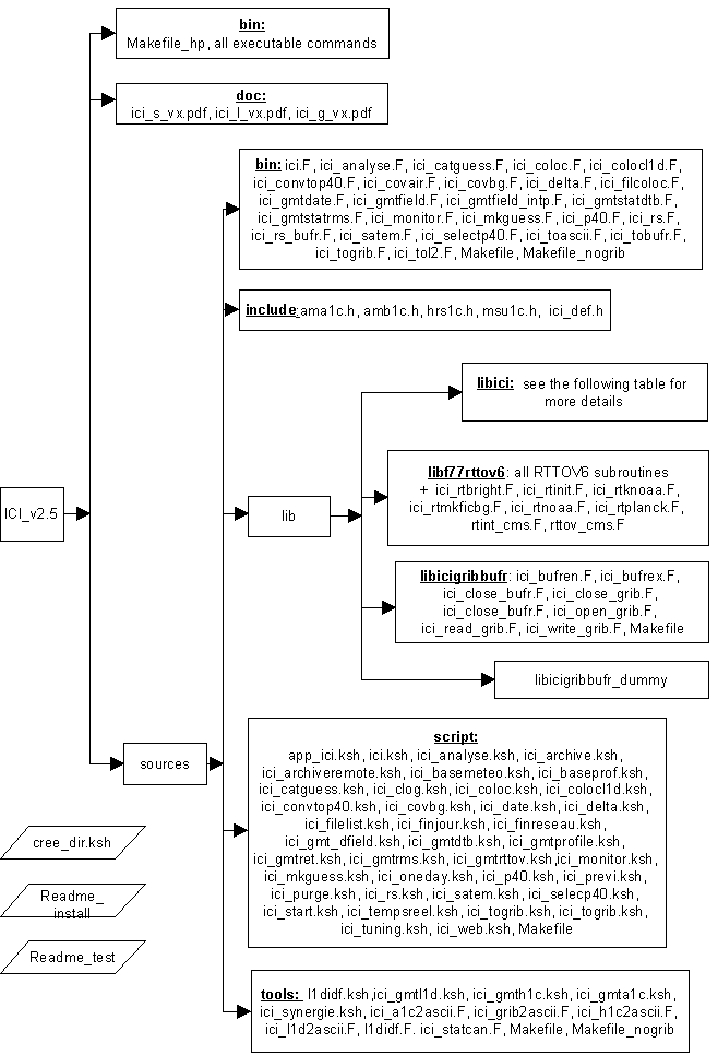The ICI application source arborescence described in the present chapter corresponds to the arborescence of the software when it was delivered.
 
Diagram -1: Source arborescence
The ICI package contains different libraries:
The libicigribbufr_dummy library contains files with same names than in the libicigribbufr library except that they invoke no routines of the Grib or the Bufr libraries. That has been done for users who do not have access to these 2 libraries.
The libf77rttov6 library contains all the routines of RTTOV6 as we get them from ECMWF and some others for the interfaces between ICI and RTTOV6.
The libici library is presented in the following table by alphabetic order. All files contains one subroutine execpt the msis.F and prfl.F files, which we get from other teams, for profile extrapolation.

airmasrs.F	airmassat.F	bd_airmasrs.F	cal_delta.F	calal.F	codebufr_atovs.F
codebufr_tovs.F	codesatem.F	coucheh2o.F	esat.F	esit.F	extr_previ.F
f_ici_ana.F	f_ici_rs.F	geogcart.F	get_refdelta.F	hutorm.F	hutotd.F
ici_calgeo.F	ici_chxl1d.F	ici_clarif.F	ici_cpl1d.F	ici_decrsbufr.F	ici_ecartprofil.F
ici_ecarttb.F	ici_elimdtb.F	ici_fn.F	ici_gmt_interpol.F	ici_gmt_smoothing.F	ici_guess.F
ici_initcan.F	ici_inv.F	ici_l1dinit.F	ici_lecl1d.F	ici_lecl1damsu.F	ici_lecl1dmsu.F
ici_level_to_field.F	ici_levels_to_fields.F	ici_msis.F	ici_nearest.F	ici_prfl.F	ici_prstn.F
ici_reglmul.F	ici_rsbufrtop40.F	ici_stat.F	ici_statchl1d.F	ici_tbguess.F	ici_tvlayers.F
ici_upg_p40.F	ici_upg_sat.F	intplog.F	lec_airmas.F	lec_cmeteo.F	lec_delta.F
lec_gmeteo.F	lec_guess.F	lec_inv.F	lec_previ.F	matcov.F	matinv.F
near_cmeteo.F	prn_cmeteo.F	prn_gmeteo.F	prn_histo.F	prn_icienv.F	prn_iciprevi.F
prn_icisat.F	prn_p40.F	profile_lay.F	rec_tropo.F	ref32po3.F	rmtohu.F
rmtotd.F	sec_numb.F	tdewi.F	tdewl.F	tdtohu.F	tdtorm.F
toth2o.F	totozone.F	tvirt.F	wr_h_l2.F	wr_rec_l2.F	ici_emis.F
ici_setup.F

Description of the content of the libici library.

 
 

2. DATA ARBORESCENCE

 

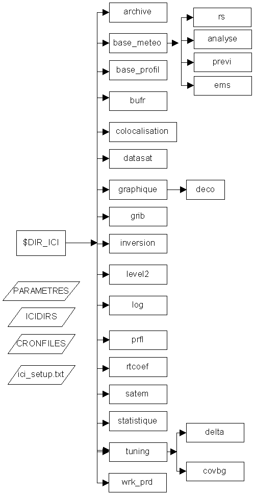
Diagram -1 : Data arborescence
The ICI application data arborescence described in this chapter corresponds to the default arborescence. It is however easy, thanks to the parametering contained in the ICIDIRS file (see Appendix 2 for details), to modify the address of a specific directory (e.g.: for the inversion directory: DIR_ICI_INV=${DIR_ICI}/toto).
The default arborescence is ${DIR_ICI} = /noaa/application/ici. Its value can be modified in the user?s ATOVS_ENV file (same as for AAPP), which is concatenated in each command of the application.
Modifying the arborescence can be useful to run the application on a double mode (e.g.: operational runs + development runs).
On the preceeding diagram, rectangulars refer to directories. Their names often explain their function. Losanges show the 3 main application?s permanent files located in the DIR_ICI directory.
This chapter details the data directories and some permanent files. The name of the directories as parametrized in the ICIDIRS file, allowing you to modify the arborescence, appears in italics.
 
/ici : DIR_ICI or ARCHIPEL_dir
Permanent files:

 
• ici_setup.txt : This file is read to set up the run conditions and contains all the channels tables depending on satellite (ex: channels used for the guess selection, for the inversion?)
• PARAMETRES: this file contains all the parameters used for launching the ICI application. For example, it contains the sampling in pixel/line of the inversion, the format of the input/output data? It can also cancel the update of internal coefficients (reinitialization of the delta_noaaxx.txt and covbg_noaaxx.mat files under /tuning)... See Appendix 1 for more details. We often refer to these parameters in the following sections.
• ICIDIRS : this file contains the parametrized names of all the directories appairing in the arborescence of diagram 3-3 just under ${DIR_ICI}.
• CRONFILE: This file can be used by the user to run the ICI software in a real-time environment. An example of the cronfile is given in Appendix 3.

 
/archive : DIR_ICI_ARCHIVE
The data arborescence under this directory for the noaaxx satellite and month yyyy_mm is : /noaaxx/yyyy_mm. It contains the main sub-directories that are stored as: base_meteo, base_profil, colocalisation, datasat, graphique, inversion, satem, statistique, tuning.
 
/base_meteo : DIR_ICI_BM
This is the residence directory for the meteorological data acquired from the GTS (Rs) worldwide time cycle or from a numerical prediction model (analysis, forecasts).
File names are always organized as follows: *_ yyyymmdd_hhmn.*, the first star representing the data type and the last star the data format, yyyy,mm,dd=year,month,day of the data, hh, mn= hour, minutes of the time cycle.
Under /base_meteo/analysis, you will find the analyses in their extraction format (e.g.:analyse*.grib) and the same ones in the p40 input format in ICI (analyse*.p40) for the requested sampling according to parametering (in the case of the CMS, it is worth 2*2, which means for the ATOUR10 grid 3,300 profiles that are 2.8MB large).
Under /base_meteo /previ you will find forecasts in their extraction format (e.g.:previ*.grib). Their name is modified to indicate the date of the forecast but their contents are not modified.
Under /base_meteo /rs you can find radiosoundings in their extraction format (e.g.:temp*.txt) and the same ones in the p40 format of input into the inversion after filtering the bad quality situations (temp*.p40).
 
/base_profil : DIR_ICI_BP
This is the residence directory for the initial library.
Names of daily files are organized as profils_noaaxx_yyyymmdd.*. Concatenated file names (ICI module input files) are as follows : profils_noaaxx.*, the star being p40, rad or tau.
info_noaaxx.txt is a small ASCII file which gives the date of the last time the rolling library was created, the number of days in depth, the selection type and sampling. If this file does not exist, the library is systematically created again. It is used for checking the current rolling library (the name of which is generic) is the one needed; its date must be the day preceding the acquisition. If the date is 99999999, the library is not created.
There are 2 permanent files under /base_profil/static :

 
• nesdispr : worldwide climatological profile file created by the NOAA/NESDIS
• satigr : worldwide climatological profile file created by the LMD team

Both files can be used in replacement of the rolling library.
 
/bufr : DIR_ICI_BUFR
This directory contains the output ICI retrieved files in bufr format when they are requested by the parametrization. They are of the form: ici_noaaxx_yyyymmdd_hhmn_nnnnn.bfs.
 
/colocalisation : DIR_ICI_CO

This is the co-locations directory. For the hhmn time cycle (with mn=00) , it contains two types of binary colocation files:

/datasat : DIR_ICI_DATASAT
This directory contains satellite data files, in the levelld format, of the form : hirsl1d_noaaxx_yyyymmdd_hhmn_nnnnn.l1d. where hhmn corresponds to the start of acquisition time, nnnnn to the orbit number. The files are compressed at the end of the inversion.

 
/graphique : DIR_ICI_GRAPHIQUE

Four permanent color palette files are under this directory: ici_temp_diff.cpt, ici_temp_rms.cpt, rttovnoaa14.cpt, rttovnoaa15.cpt. They are used by the ici_gmt* commands.
This directory contains all the postcript files produced by the ici_gmt commands. The name of each file contains the date related to the figure (ex: rms_period_noaaxx_all_yyyymmdd_mask.ps).
The directory also contains gif files, with a generic name without the date inside: these files are sent by ftp to a web server which is very limited in disk space. Use of generic names is a sure way not to increase the number of files and consequently the used space on the disk. And there is no necessity to purge the files. (ex: rms_year_noaaxx_mask.gif).
An html permanent file: validation.html is also in the directory for the vizualisation of the different gifs in the same way than under the ICI web site. Under the /deco sub-directory, we also have put a permanent file sail_bar.gif invoked by validation.html, just for the ?fun? (and to have exactly the same page than under the ICI web site.

 
/grib : DIR_ICI_GRIB
This directory contains the output ICI retrieved files in grib format when they are requested by the parametrization. They are of the form: ici_noaaxx_yyyymmdd_hhmn.grib.
 
/inversion : DIR_ICI_INV

This directory contains the binary files resulting from the inversion of the form: ici_noaaxx_yyyymmdd_hhmn_nnnnn.ici. If you have requested ascii formatted files from inverted files, you will find them in this directory under the following name: ici_noaaxx_yyyymmdd_hhmn_nnnnn.txt

 
/level2 :DIR_ICI_LEVEL2
This directory contains the output ICI retrieved files in AAPP level2 ASCII format when they are requested by the parametrization.
 
/log : DIR_ICI_LOG
This directory contains all the run logs of the ICI application.
 
/prfl : DIR_ICI_PRFL
It contains the 2 MESO_da and MOBIDIC_da permanent files  with ozone climatological profiles and also for profile extrapolation, when requested by parametrization.
 
/rtcoef : DIR_ICI_RTNOAA
This directory is linked to the radiative transfer model with the permanent rt_coef_noaa.dat file (presently for the RTTOV6 release). This file contains the coefficients required for running the direct RTTOV model, in particular for all satellites, the central frequencies of the channels, the internal statistic coefficients required for the fast model and contains the values required for computing the micro-wave emissivity on sea in relation to the wind velocity.
 
/satem :DIR_ICI_SATEM
It contains the output ICI retrieved files in SATEM format when requested by the parametrization.

/statistique :DIR_ICI_STAT
This directory contains the bias and standard deviation statistics files computed by using the coloc_noaaxx*.ici files. Filenames are as follows : statici_noaaxx_all_yyyymmdd_hhmn.txt or statici_noaaxx_rs_yyyymmdd_hhmn.txt (with radiosonde only),with hhmn the time cycle. For several days at a time (10 being the default value) they are named statici_noaaxx_all_yyyymmdd_yyyymmdd.txt or statici_noaaxx_rs_yyyymmdd_yyyymmdd.txt. In previous V2 version, the name of the files were deltaici* (same files).
 
/tuning : DIR_ICI_TUNING
This is the residence arborescence with 2 sub-directories one for the error covariance matrix files of the initial profile (/covbg), the second for the ascii files for all the biases (/delta).
Under /tuning/covbg, file names between two dates are as follows :

Under /tuning/delta, file names are follows:

Under /tuning, we found the statistical files used in input of the ici command.They are generated through a copy of the preceeding files for the correct dates, with a generic name. They are:

/wrk_prd: : DIR_ICI_TMP
Several commands are executed on a tempory directory, which is defined at the start of command. The directory is of the following type: ${DIR_ICI}/wrk_prd/cmd_pid where cmd is the name of the command and pid the number of the process under way (expansion of the $$ shell). At the end of the command the directory is emptied except for a file called ici_working and the directory is purged by means of the general purge command. Here is the list of the commands that use a work directory:
app_ici ici ici_analyse ici_baseprof ici_coloc ici_colocl1d ici_covbg
ici_delta ici_gmt* ici_monitor ici_rs ici_satem ici_togrib ici_tuning
ici_start
 

 
1. I/O INTERFACES

Most files have a sequential access and no header. It is therefore possible to concatenate them in order to obtain files on longer periods of time for example. File sizes are specified for noaa15 (larger than for Noaa14) and for CMS acquisition zone.
 

 
1. files for a PASS processing

app_ici input files

 
• set_up.txt, PARAMETRES and ICIDIRS under ${DIR_ICI} for the run conditions.

 
• hirsl1d_noaaxx_yyyymmdd_hhmn_nnnnn.l1d. under /datasat. This is the satellite data file. Its format is specified in [3]. The ICI application uses the following data:

It is about 1.8MB size wise and 1MB when compressed.

 
• previ_noaaxx_yyyymmdd_hhmn.grib. under /base_meteo/previ. This file contains the forecasts in grib format. The data that can be used for inversion are: Pmer, T1000hpa, Z1000hpa U2m and V2m. 1MB.

 
• delta_noaaxx.txt. under /tuning. Statistics file, 40KB. It is an ASCII file located under the /tuning directory. Each line is self-documented by the 1^st word on the line (e.g. :SDTB). For word definition, see description of ici_delta files in this section.

 
• covbg_noaaxx.mat. under /tuning. It is the error covariance matrix file for the initial profile. 220KB.

 
• profils_noaaxx.p40. under /base_profil. It is the profiles file from the initial library.1.28 MB

 
• profils_noaaxx.rad. under /base_profil. It is the up and down radiances file from the initial library. 49.6 MB

 
• profils_noaaxx.tau. under /base_profil. It is the total transmittances file from the initial library. 28 MB

 
• covair_noaaxx.mat. under /base_profil. It is the file containing the air mass covariance matrixes related to the initial library. 220KB.

 
• rt_coef_noaa.dat under /rtcoef. It is the RTTOV internal coefficients file which is necessary as soon as RTTOV has to be used. It is also used by the commands ici_baseprof, ici_delta, ici_monitor, ici_mkguess. This file now contains the coefficients required for computing the micro-wave surface emissivity on sea (in a separate file in previous ici version). 3.6MB

 
app_ici output files

 
• ici_noaaxx_yyyymmdd_hhmn_nnnnn.ici file of binary format inversions. under /inversion. This sequential access binary file can reach 4.5MB for an orbit at a 1-pixel/2, 1-line/2 resolution. Each record contains:

Structures are described in appendix 4.

 
• stm_noaaxx_yyyymmdd_hhmn_nnnnn_no.txt satem format inversions file. under /satem. These files only exist when requested by means of the parametering PAR_ICI_SATEM. File format is defined by the OMM FM 86 code completed with the Transmet header. Each file contains a maximum of 99 messages (1 per situation) with a total of up to 10 files (numbered from 01 to 10) for an orbit inverted at the 1-pixel/2, 1-line/2 resolution. Each record contains:

 
• ici_noaaxx_yyyymmdd_hhmm_nnnnn.txt ascii format inversions file. under /inversion. This format is now mainly used for co-locations description because the ascii level2 format has been defined as a standard of level2 files for Eumetsat softwares. This format contains :

 
 
 

satellite name	orbit number
date of HIRS spot	lat, lon, alt	satellite zenithal angle	land/sea/coast	HIRS channels	AMSU/MSU channels
Tsurface	clear percentage	cloud top temperature	surface pressure
profile type :  rs, analysis, inversion	Rs code	date of profile	profile?s lat,lon,alt	land/sea index
temperature of the 40-level profile	water vapor on the 25 lower levels

 
• ici_noaaxx_yyyymmdd_hh00.grib grib format inversions file. under /grib If parametering requires it, for each orbit a grib file is produced (at the end of the app_ici command) or either for the concatenation of the 3 or 4 successive orbits by calling the ici_togrib command by crontab. The file size can reach 2MB for 3 concatenated orbits. The hh00 corresponds to the nearest hour from the orbit time.

 
• ici_noaaxx_yyyymmdd_hhmn_nnnnn.bfs Bufr format inversion file. Under /bufr. It is a standard WMO format and is now used by CMS to provide the ICI retrievals to theFrench Met Service for NWP monitoring. About 100KB for a 2x2 resolution.

 
• AAPP level2 format inversions file. If it is requested by parametering, it is possible to activate the coding in the AAPP level2 format by means of the ici_tol2.F routine. The file format is described in Appendix 8.

 
• ici_noaaxx_yyyymmdd_hhmn_nnnnn.log inversion processing log file. Under /log. It contains all the print-outs performed while running ici.F, in particular the running conditions for each situation. This file can be quite large and it is systematically compressed at the end of running. It can reach 5MB when compressed.

 
1. files for the BASE_METEO creation

ici_analyse, ici_previ, ici_rs input files
If the data is acquired in the GRIB format (PAR_ICI_ANAFMT=GRIB or PAR_ICI_PREFMT=GRIB), the original files of the meteorological base for analyses or forecasts are located in a directory parametered as DIR_ICI_ANAGRIB for analyses and DIR_ICI_PREGRIB for forecasts. Analyses and Forecasts should contain the grid-related surface parameters (land/sea and altitude). If these fields arein a separate file (as it is the case at CMS), under DIR_ICI_CSTGRIB, the scripts ici_analyse and ici_previ make first the concatenation of the 2 files.
If the data is acquired in the ASCII format (format (PAR_ICI_ANAFMT=ASCII or PAR_ICI_PREFMT=ASCII), the original files of the meteorological base are located in a directory parametered as DIR_ICI_ANAASCII for analyses and DIR_ICI_PREVIASCII for forecasts. The files contain the grid-related surface parameters (land/sea and altitude).
Radio soundings are located under DIR_ICI_RSASCII for ASCII format. In case of BUFR format, the residence of the radiosondings will be under DIR_ICI_RSBUFR .
All these directories are located on a machine which is directly connected with the numerical prediction center (e.g.:Arpège at CMS). Residence of original files and their names and formats obviously depend very much on the acquisition center.
 
ici_analyse output files

 
• analyse_yyyymmdd_hh00.p40 analyses in the p40 format. Under ${DIR_ICI_BM}/analyse. This file is sequential and binary. It contains 1 profile per record. Each analysis is encoded in the p40 format which can be read by RTTOV. The p40 format is indicated in appendix 4 (ici_def.h). This file may contain less situations than the input file analyse*.grib, depending on the adopted parametering PAR_ICI_ANAECHP and PAR_ICI_ANAECHL. For the ATOUR 10 grid with a sampling every 2 degrees : 2.8MB.

 
• analyse_yyyymmdd_hh00.grib analyses in the grib format.The analyses of the general directory DIR_ICI_ANAGRIB are copied into ${DIR_ICI_BM}/analyse. Retrieved analyses are in the GRIB format with 1 parameter per field. The format depends on the HRPT center and will probably be different for another user. For the ATOUR10 grid, 1MB. 4 per day.

ici_previ output files

 
• previ_yyyymmdd_hh00.grib forecasts in the grib format. Under ${DIR_ICI_BM}/previ. forecasts from the DIR_ICI_PREGRIB directory are copied into ${DIR_ICI_BM}/previ. The date and time corresponding to the time cycle for which the forecast is valid. 1MB, 4 per day.

ici_rs output files
output

 
• temp_yyyymmdd_hh00.p40. Under ${DIR_ICI_BM}/rs. This file contains the rs after filtering and coding in the p40 format. E.g.:110KB for the 00-h time cycle.

 
• yyyymmddhh00.Z radiosondings in the bufr format. Radio soundings from DIR_ICI_RSBUFR are copied and compressed into ${DIR_ICI_BM}/rs.

 
1. Files for the BASE_PROFIL initial library

ici_mkguess
input

 
• analyse_yyyymmdd_hh00.p40 under /base_meteo/analyse, hh depends on parametrization (00 at CMS today).

output

 
• profils_noaaxx_yyyymmdd.p40, under /base_profil. Binary daily file with direct profile access in the p40 format. Ex: 128KB for the ATOUR10 area, on a 10*10 degrees grid.

 
• profils_noaaxx_yyyymmdd.rad, under /base_profil. Binary daily file with direct access of the up and down radiances corresponding to the preceding profiles. Indexing depends on ground pressure and on the secant, each record containing the values for all profiles and channels. 5MB

 
• profils_noaaxx_yyyymmdd.tau, under /base_profil. Binary daily file with direct access containing the total transmittances corresponding to the preceding profiles. 2.5MB

ici_catguess
input

 
• profils_noaaxx_yyyymmdd.p40, under /base_profil.
• profils_noaaxx_yyyymmdd.rad, under /base_profil.

 
• profils_noaaxx_yyyymmdd.tau, under /base_profil.

output

 
• profils_noaaxx.p40, under /base_profil. contains the profiles in the initial library. 1.28MB

 
• profils_noaaxx.rad, under /base_profil. contains the up and down radiances in the initial library. 49.6MB

 
• profils_noaaxx.tau, under /base_profil. contains the total transmittances in the initial library. 28MB

 
ici_covair.exe
input

 
• profils_noaaxx.rad, under /base_profil

output

 
• covair_noaaxx.mat, under /base_profil. Contains the covariance matrixes of the Tbs computed from the profils_noaaxx.rad. file 23KB

 
ici_baseprof output files

 
• info_noaaxx.txt , under /base_profil. ascii file that contains information on the initial library

 
• baseprof_ yyyymmdd.log , under /log. contains information on the run

 
1. MONITORING files

Warning: Two different lines of statistics exist:

 
1. RTTOV forward biases from colocalions of in-situ profiles with l1d files by using the command serie: ici_colocl1d (colocl1d*.ici) -> ici_delta (delta_noaaxx*.txt) -> ici_tuning (delta_noaaxx.txt). The delta_noaaxx.txt is the statistic tuning file in input of ici command.
2. ICI statistics from colocations of in-situ profiles with ici inversion files by using the command serie: ici_coloc (coloc_noaaxx*.ici) ->

ici_colocl1d input files
input

 
• hrsl1d_noaaxx_yyyymmdd_hhmn_nnnnn.l1d files under /datasat (output file of AAPP)

 
• analyse_yyyymmdd_hh00.p40 under /base_meteo/analyse

 
• temp_yyyymmdd_hh00.p40 under /base_meteo/rs

output

 
• colocl1d_noaaxx_yyyymmdd_hhmn_nnnnn.ici, under /colocalisation, co-location file for a pass. Sequential access and binary. Each file can reach 600KB. Each record contains information from the l1d file and from the colocated analyse* or temp* profile.

 
ici_coloc input files
input

 
• ici_noaaxx_yyyymmdd_hhmn_nnnnn.ici files under /inversion (output files for the ici command)

 
• analyse_yyyymmdd_hh00.p40 under /base_meteo/analyse

 
• temp_yyyymmdd_hh00.p40 under /base_meteo/rs

output

 
• coloc_noaaxx_yyyymmdd_hh00.ici, under /colocalisation, co-location file for a hh time cycle. sequential access and binary. Each file can reach 3MB. Each record contains information from the ici*.ici file and from the co-located profile analyse* or temp* file, i.e.:

ici_delta
input

 
• colocl1d_noaaxx_yyyymmdd_hhmn_nnnnn.ici all the files concatenated as asked by parametrization (ex: all orbits of a cycle)

output

 
• delta_noaaxx_type_yyyymmdd_hh00.txt. under /tuning/delta. It is an ascii file containing the statistics for the concatenation of 2 time cycles hh and hh+06h

 
• delta_noaaxx_type_yyyymmdd_yyyymmdd.txt. under /tuning/delta. it contains the statistics for the concatenation of all time cycles between the 2 dates appearing in the name. type= all (for all profile type) or rs. 40KB.

Each type of statistics has an identifier in the first column, preceded by M for mean, S for standard deviation and N for number of values. This way, identifier DTB will be allocated to the mean of the deviations between synthetic brightness temperatures and the temperatures measured by the instrument (before any correction). The next columns hold the starting date (yyyymmdd), ending date (yyyymmdd), time cycle (hh or 99), satellite name, then the computing type (land/sea, clear index, secant) followed by the actual values. Patterns are defined in description of ici_delta.F.
The file also contains information lines on the columns (channel numbers) so as to easily create time-division files containing the same type of information arranged in columns, in particular for tracing these values.

ici_monitor
input

 
• coloc_noaaxx_yyyymmdd_hh00.ici all the files concatenated as asked by parametrization

output

 
• statici_noaaxx_type_yyyymmdd_hh00.txt. under /statistique. It is an ascii file containing the statistics for the concatenation of 2 time cycles hh and hh+06h

 
• statici_noaaxx_type_yyyymmdd_yyyymmdd.txt. under /statistique. it contains the statistics for the concatenation of all time cycles between the 2 dates appearing in the name. 80KB.

ici_covbg
input

 
• coloc_noaaxx_yyyymmdd_hh00.ici all the files concatenated as asked by parametrization

output

 
• covbg_noaaxx_yyyymmdd_yyyymmdd.mat under /tuning/covbg. Binary file containing the error covariance matrix of the initial profile.220KB.

 
ici_tuning
input

 
• colocl1d_noaaxx_yyyymmdd_hhmn_nnnnn.ici all the files concatenated as asked by parametrization
• coloc_noaaxx_yyyymmdd_hh00.ici all the files concatenated as asked by parametrization

output

 
• delta_noaaxx_type_yyyymmdd_yyyymmdd.txt. under /tuning/delta. it contains the statistics (from l1d files) for the concatenation of all time cycles between the 2 dates appearing in the name. type= all and rs (2 files). 40KB each.

 
• statici_noaaxx_type_yyyymmdd_yyyymmdd.txt. under /statistique. it contains the statistics (from ici inversion files) for the concatenation of all time cycles between the 2 dates appearing in the name. type= all and rs (2 files). 80KB each.

 
• covbg_noaaxx_yyyymmdd_yyyymmdd.mat under /tuning/covbg. Binary file containing the error covariance matrix of the initial profile.220KB.

 
• delta_noaaxx.txt. under /tuning. This is the statistics file on input of the ici. command with a generic name, copy of a file delta_noaaxx_all_yyyymmdd_yyyymmdd.txt having the proper dates

 
• covbg_noaaxx.mat. under /tuning. This is the guess?s error covariance matrix on input of the ici command with a generic name, copy of a file covbg_noaaxx_yyyymmdd_yyyymmdd.mat having the proper dates

 
• info_noaaxx.txt. under /tuning. It is an ascii file containing information on tuning

 
1. GRAPHIC files

ici_web
comment: ici_web calls several individual graphic commands of the form ici_gmt* which can be called alone. The main difficulty with GMT software is that the graphic output files are in postcript format and another tool is needed to convert them in gif format for their visualization on http.
inputs

 
• under ${DIR_ICI_GRAPHIQUE} : ici_temp_diff.cpt ici_temp.cpt ici_temp_rms.cpt rttovnoaaxx.cpt
• under ${DIR_ICI_INV} : ici_noaaxx_yyyymmdd_*_*.ici
• under ${DIR_ICI_BM}/analyse: analyse_yyyymmdd_hh00.p40
• under ${DIR_ICI_STAT}: statici_noaaxx_all_yyymmdd_yyyymmdd.txt

outputs under ${DIR_ICI_GRAPHIQUE}
POSTCRIPT files of the different figures. Sizes are given as a reference but of course depend on the processed situation. The name of each command is given in front of each postcript file which is an output of this command.

 
• dtb_period_noaaxx_type_yyyymmdd_mask_n.ps 88KB ici_gmtdtb
• icidiff_yyyymmdd_hh_valplev.ps 600KB ici_gmt_dtfield
• rttov_noaaxx_yyyymmdd_mask.ps 22KB ici_gmtrttov
• rms_period_noaaxx_type_yyyymmdd_mask.ps 3MB ici_gmtrms
• ici_noaaxx_yyyymmdd_hh_${param}plevel.ps 1MB ici_gmtret
• profile_noaaxx_type_yyyymmdd_${rettype}${paramtype}.ps 35KB ici_gmtprofile

GIF corresponding generic files

 
• icidiff_noaaxx_ppp.gif ppp= 500, 700, 850, 1000 40KB each
• profile_noaaxx_type.gif type= all and rs 12KB
• rms_2months_noaaxx_all_mask.gif 60KB
• rms_year_noaaxx_type_mask.gif type= all in this version 30KB
• rttov_noaaxx.gif 7KB
• dtb_2months_noaaxx_all_n.gif 20KB each
• dtb_year_noaaxx_type_n.gif n=1,4 for ATOVS type= all in this version 20KB each